skopt.plots.plot_objective
-
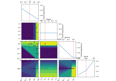
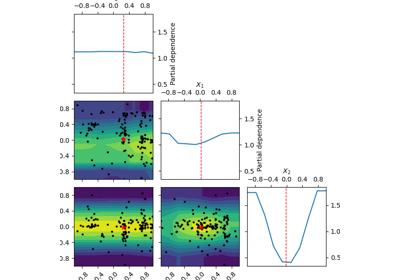
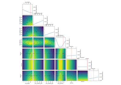
skopt.plots.plot_objective(result, levels=10, n_points=40, n_samples=250, size=2, zscale='linear', dimensions=None, sample_source='random', minimum='result', n_minimum_search=None, plot_dims=None, show_points=True, cmap='viridis_r')[source][source]¶ Plot a 2-d matrix with so-called Partial Dependence plots of the objective function. This shows the influence of each search-space dimension on the objective function.
This uses the last fitted model for estimating the objective function.
The diagonal shows the effect of a single dimension on the objective function, while the plots below the diagonal show the effect on the objective function when varying two dimensions.
The Partial Dependence is calculated by averaging the objective value for a number of random samples in the search-space, while keeping one or two dimensions fixed at regular intervals. This averages out the effect of varying the other dimensions and shows the influence of one or two dimensions on the objective function.
Also shown are small black dots for the points that were sampled during optimization.
A red star indicates per default the best observed minimum, but this can be changed by changing argument ´minimum´.
Note
The Partial Dependence plot is only an estimation of the surrogate model which in turn is only an estimation of the true objective function that has been optimized. This means the plots show an “estimate of an estimate” and may therefore be quite imprecise, especially if few samples have been collected during the optimization (e.g. less than 100-200 samples), and in regions of the search-space that have been sparsely sampled (e.g. regions away from the optimum). This means that the plots may change each time you run the optimization and they should not be considered completely reliable. These compromises are necessary because we cannot evaluate the expensive objective function in order to plot it, so we have to use the cheaper surrogate model to plot its contour. And in order to show search-spaces with 3 dimensions or more in a 2-dimensional plot, we further need to map those dimensions to only 2-dimensions using the Partial Dependence, which also causes distortions in the plots.
- Parameters
- result
OptimizeResult The optimization results from calling e.g.
gp_minimize().- levelsint, default=10
Number of levels to draw on the contour plot, passed directly to
plt.contourf().- n_pointsint, default=40
Number of points at which to evaluate the partial dependence along each dimension.
- n_samplesint, default=250
Number of samples to use for averaging the model function at each of the
n_pointswhensample_methodis set to ‘random’.- sizefloat, default=2
Height (in inches) of each facet.
- zscalestr, default=’linear’
Scale to use for the z axis of the contour plots. Either ‘linear’ or ‘log’.
- dimensionslist of str, default=None
Labels of the dimension variables.
Nonedefaults tospace.dimensions[i].name, or if alsoNoneto['X_0', 'X_1', ..].- plot_dimslist of str and int, default=None
List of dimension names or dimension indices from the search-space dimensions to be included in the plot. If
Nonethen use all dimensions except constant ones from the search-space.- sample_sourcestr or list of floats, default=’random’
Defines to samples generation to use for averaging the model function at each of the
n_points.A partial dependence plot is only generated, when
sample_sourceis set to ‘random’ andn_samplesis sufficient.sample_sourcecan also be a list of floats, which is then used for averaging.Valid strings:
‘random’ -
n_samplesrandom samples will used‘result’ - Use only the best observed parameters
‘expected_minimum’ - Parameters that gives the best minimum Calculated using scipy’s minimize method. This method currently does not work with categorical values.
‘expected_minimum_random’ - Parameters that gives the best minimum when using naive random sampling. Works with categorical values.
- minimumstr or list of floats, default = ‘result’
Defines the values for the red points in the plots. Valid strings:
‘result’ - Use best observed parameters
‘expected_minimum’ - Parameters that gives the best minimum Calculated using scipy’s minimize method. This method currently does not work with categorical values.
‘expected_minimum_random’ - Parameters that gives the best minimum when using naive random sampling. Works with categorical values
- n_minimum_searchint, default = None
Determines how many points should be evaluated to find the minimum when using ‘expected_minimum’ or ‘expected_minimum_random’. Parameter is used when
sample_sourceand/orminimumis set to ‘expected_minimum’ or ‘expected_minimum_random’.- show_points: bool, default = True
Choose whether to show evaluated points in the contour plots.
- cmap: str or Colormap, default = ‘viridis_r’
Color map for contour plots. Passed directly to
plt.contourf()
- result
- Returns
- ax
Matplotlib.Axes A 2-d matrix of Axes-objects with the sub-plots.
- ax