Note
Click here to download the full example code or to run this example in your browser via Binder
Partial Dependence Plots
Sigurd Carlsen Feb 2019 Holger Nahrstaedt 2020
Plot objective now supports optional use of partial dependence as well as different methods of defining parameter values for dependency plots.
print(__doc__)
import sys
from skopt.plots import plot_objective
from skopt import forest_minimize
import numpy as np
np.random.seed(123)
import matplotlib.pyplot as plt
Objective function
Plot objective now supports optional use of partial dependence as well as different methods of defining parameter values for dependency plots
# Here we define a function that we evaluate.
def funny_func(x):
    s = 0
    for i in range(len(x)):
        s += (x[i] * i) ** 2
    return s
Optimisation using decision trees
We run forest_minimize on the function
bounds = [(-1, 1.), ] * 3
n_calls = 150

result = forest_minimize(funny_func, bounds, n_calls=n_calls,
                         base_estimator="ET",
                         random_state=4)
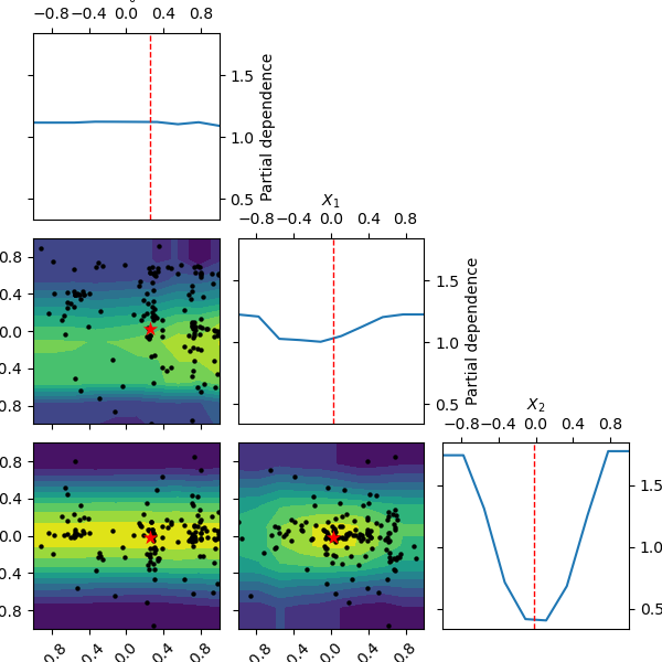
Partial dependence plot
Here we see an example of using partial dependence. Even when setting n_points all the way down to 10 from the default of 40, this method is still very slow. This is because partial dependence calculates 250 extra predictions for each point on the plots.
_ = plot_objective(result, n_points=10)
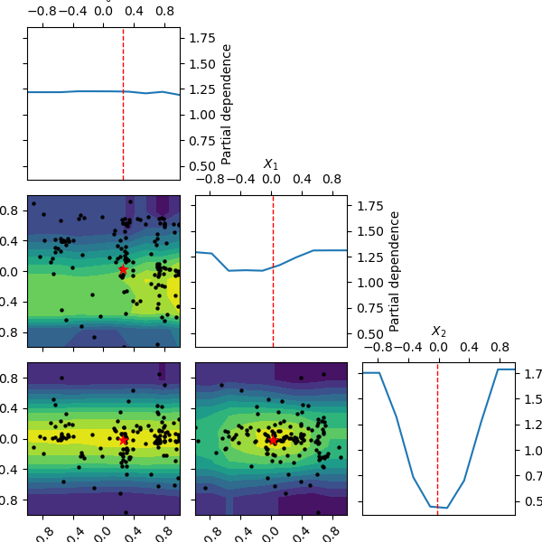
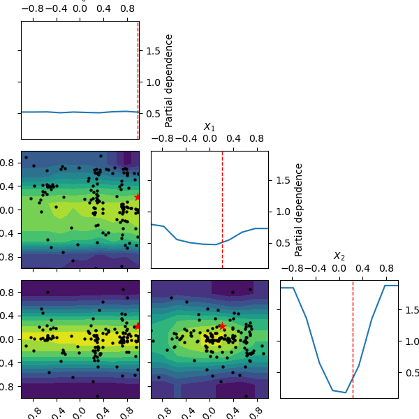
It is possible to change the location of the red dot, which normally shows the position of the found minimum. We can set it ‘expected_minimum’, which is the minimum value of the surrogate function, obtained by a minimum search method.
_ = plot_objective(result, n_points=10, minimum='expected_minimum')
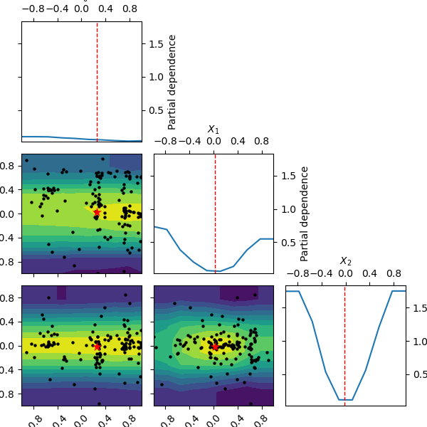
Plot without partial dependence
Here we plot without partial dependence. We see that it is a lot faster. Also the values for the other parameters are set to the default “result” which is the parameter set of the best observed value so far. In the case of funny_func this is close to 0 for all parameters.
_ = plot_objective(result, sample_source='result', n_points=10)

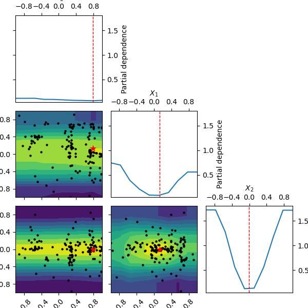
Modify the shown minimum
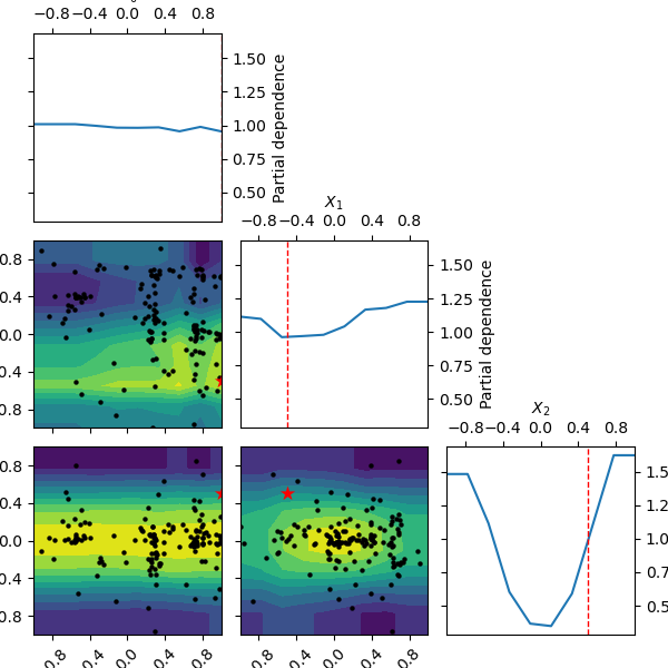
Here we try with setting the minimum parameters to something other than
“result”. First we try with “expected_minimum” which is the set of
parameters that gives the miniumum value of the surrogate function,
using scipys minimum search method.
_ = plot_objective(result, n_points=10, sample_source='expected_minimum',
                   minimum='expected_minimum')
“expected_minimum_random” is a naive way of finding the minimum of the surrogate by only using random sampling:
_ = plot_objective(result, n_points=10, sample_source='expected_minimum_random',
                   minimum='expected_minimum_random')
We can also specify how many initial samples are used for the two different “expected_minimum” methods. We set it to a low value in the next examples to showcase how it affects the minimum for the two methods.
_ = plot_objective(result, n_points=10, sample_source='expected_minimum_random',
                   minimum='expected_minimum_random',
                   n_minimum_search=10)
_ = plot_objective(result, n_points=10, sample_source="expected_minimum",
                   minimum='expected_minimum', n_minimum_search=2)

Set a minimum location
Lastly we can also define these parameters ourself by parsing a list as the minimum argument:
_ = plot_objective(result, n_points=10, sample_source=[1, -0.5, 0.5],
                   minimum=[1, -0.5, 0.5])
Total running time of the script: ( 0 minutes 45.822 seconds)
Estimated memory usage: 8 MB