Note
Click here to download the full example code or to run this example in your browser via Binder
Comparing initial point generation methods
Holger Nahrstaedt 2020
Bayesian optimization or sequential model-based optimization uses a surrogate
model to model the expensive to evaluate function func. There are several
choices for what kind of surrogate model to use. This notebook compares the
performance of:
Halton sequence,
Hammersly sequence,
Sobol sequence and
Latin hypercube sampling
as initial points. The purely random point generation is used as a baseline.
print(__doc__)
import numpy as np
np.random.seed(123)
import matplotlib.pyplot as plt
Toy model
We will use the benchmarks.hart6 function as toy model for the expensive function.
In a real world application this function would be unknown and expensive
to evaluate.
from skopt.benchmarks import hart6 as hart6_
# redefined `hart6` to allow adding arbitrary "noise" dimensions
def hart6(x, noise_level=0.):
    return hart6_(x[:6]) + noise_level * np.random.randn()

from skopt.benchmarks import branin as _branin

def branin(x, noise_level=0.):
    return _branin(x) + noise_level * np.random.randn()
from matplotlib.pyplot import cm
import time
from skopt import gp_minimize, forest_minimize, dummy_minimize

def plot_convergence(result_list, true_minimum=None, yscale=None, title="Convergence plot"):

    ax = plt.gca()
    ax.set_title(title)
    ax.set_xlabel("Number of calls $n$")
    ax.set_ylabel(r"$\min f(x)$ after $n$ calls")
    ax.grid()
    if yscale is not None:
        ax.set_yscale(yscale)
    colors = cm.hsv(np.linspace(0.25, 1.0, len(result_list)))

    for results, color in zip(result_list, colors):
        name, results = results
        n_calls = len(results[0].x_iters)
        iterations = range(1, n_calls + 1)
        mins = [[np.min(r.func_vals[:i]) for i in iterations]
                for r in results]
        ax.plot(iterations, np.mean(mins, axis=0), c=color, label=name)
        #ax.errorbar(iterations, np.mean(mins, axis=0),
        #             yerr=np.std(mins, axis=0), c=color, label=name)
    if true_minimum:
        ax.axhline(true_minimum, linestyle="--",
                   color="r", lw=1,
                   label="True minimum")
    ax.legend(loc="best")
    return ax


def run(minimizer, initial_point_generator,
        n_initial_points=10, n_repeats=1):
    return [minimizer(func, bounds, n_initial_points=n_initial_points,
                      initial_point_generator=initial_point_generator,
                      n_calls=n_calls, random_state=n)
            for n in range(n_repeats)]


def run_measure(initial_point_generator, n_initial_points=10):
    start = time.time()
    # n_repeats must set to a much higher value to obtain meaningful results.
    n_repeats = 1
    res = run(gp_minimize, initial_point_generator,
              n_initial_points=n_initial_points, n_repeats=n_repeats)
    duration = time.time() - start
    # print("%s %s: %.2f s" % (initial_point_generator,
    #                          str(init_point_gen_kwargs),
    #                          duration))
    return res
Objective
The objective of this example is to find one of these minima in as
few iterations as possible. One iteration is defined as one call
to the benchmarks.hart6 function.
We will evaluate each model several times using a different seed for the random number generator. Then compare the average performance of these models. This makes the comparison more robust against models that get “lucky”.
from functools import partial
example = "hart6"

if example == "hart6":
    func = partial(hart6, noise_level=0.1)
    bounds = [(0., 1.), ] * 6
    true_minimum = -3.32237
    n_calls = 40
    n_initial_points = 10
    yscale = None
    title = "Convergence plot - hart6"
else:
    func = partial(branin, noise_level=2.0)
    bounds = [(-5.0, 10.0), (0.0, 15.0)]
    true_minimum = 0.397887
    n_calls = 30
    n_initial_points = 10
    yscale="log"
    title = "Convergence plot - branin"
from skopt.utils import cook_initial_point_generator

# Random search
dummy_res = run_measure("random", n_initial_points)
lhs = cook_initial_point_generator(
    "lhs", lhs_type="classic", criterion=None)
lhs_res = run_measure(lhs, n_initial_points)
lhs2 = cook_initial_point_generator("lhs", criterion="maximin")
lhs2_res = run_measure(lhs2, n_initial_points)
sobol = cook_initial_point_generator("sobol", randomize=False,
                                     min_skip=1, max_skip=100)
sobol_res = run_measure(sobol, n_initial_points)
halton_res = run_measure("halton", n_initial_points)
hammersly_res = run_measure("hammersly", n_initial_points)
grid_res = run_measure("grid", n_initial_points)
Note that this can take a few minutes.
plot = plot_convergence([("random", dummy_res),
                        ("lhs", lhs_res),
                        ("lhs_maximin", lhs2_res),
                        ("sobol", sobol_res),
                        ("halton", halton_res),
                        ("hammersly", hammersly_res),
                        ("grid", grid_res)],
                        true_minimum=true_minimum,
                        yscale=yscale,
                        title=title)

plt.show()
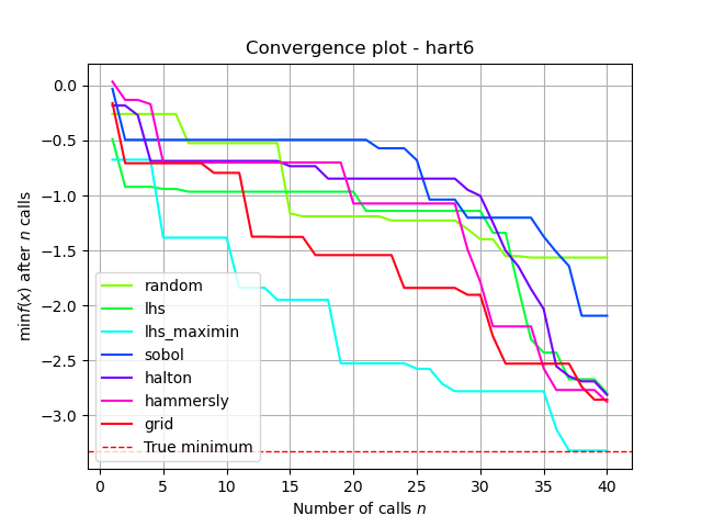
This plot shows the value of the minimum found (y axis) as a function
of the number of iterations performed so far (x axis). The dashed red line
indicates the true value of the minimum of the benchmarks.hart6
function.
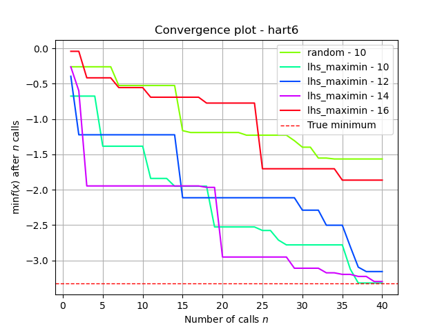
Test with different n_random_starts values
lhs2 = cook_initial_point_generator("lhs", criterion="maximin")
lhs2_15_res = run_measure(lhs2, 12)
lhs2_20_res = run_measure(lhs2, 14)
lhs2_25_res = run_measure(lhs2, 16)
n_random_starts = 10 produces the best results
plot = plot_convergence([("random - 10", dummy_res),
                        ("lhs_maximin - 10", lhs2_res),
                        ("lhs_maximin - 12", lhs2_15_res),
                        ("lhs_maximin - 14", lhs2_20_res),
                        ("lhs_maximin - 16", lhs2_25_res)],
                        true_minimum=true_minimum,
                        yscale=yscale,
                        title=title)

plt.show()
Total running time of the script: ( 2 minutes 50.755 seconds)
Estimated memory usage: 8 MB