Note
Click here to download the full example code or to run this example in your browser via Binder
Use different base estimators for optimization
Sigurd Carlen, September 2019. Reformatted by Holger Nahrstaedt 2020
To use different base_estimator or create a regressor with different parameters, we can create a regressor object and set it as kernel.
This example uses plots.plot_gaussian_process which is available
since version 0.8.
print(__doc__)

import numpy as np
np.random.seed(1234)
import matplotlib.pyplot as plt
from skopt.plots import plot_gaussian_process
from skopt import Optimizer
Toy example
Let assume the following noisy function \(f\):
noise_level = 0.1

# Our 1D toy problem, this is the function we are trying to
# minimize


def objective(x, noise_level=noise_level):
    return np.sin(5 * x[0]) * (1 - np.tanh(x[0] ** 2))\
           + np.random.randn() * noise_level


def objective_wo_noise(x):
    return objective(x, noise_level=0)
opt_gp = Optimizer([(-2.0, 2.0)], base_estimator="GP", n_initial_points=5,
                acq_optimizer="sampling", random_state=42)
def plot_optimizer(res, n_iter, max_iters=5):
    if n_iter == 0:
        show_legend = True
    else:
        show_legend = False
    ax = plt.subplot(max_iters, 2, 2 * n_iter + 1)
    # Plot GP(x) + contours
    ax = plot_gaussian_process(res, ax=ax,
                               objective=objective_wo_noise,
                               noise_level=noise_level,
                               show_legend=show_legend, show_title=True,
                               show_next_point=False, show_acq_func=False)
    ax.set_ylabel("")
    ax.set_xlabel("")
    if n_iter < max_iters - 1:
        ax.get_xaxis().set_ticklabels([])
    # Plot EI(x)
    ax = plt.subplot(max_iters, 2, 2 * n_iter + 2)
    ax = plot_gaussian_process(res, ax=ax,
                               noise_level=noise_level,
                               show_legend=show_legend, show_title=False,
                               show_next_point=True, show_acq_func=True,
                               show_observations=False,
                               show_mu=False)
    ax.set_ylabel("")
    ax.set_xlabel("")
    if n_iter < max_iters - 1:
        ax.get_xaxis().set_ticklabels([])
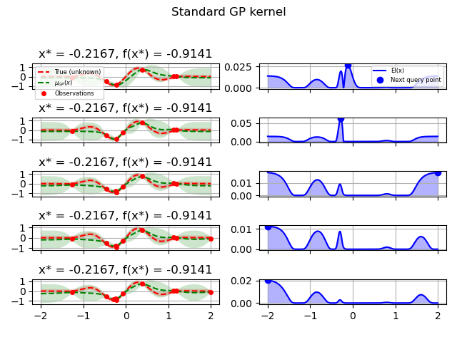
GP kernel
fig = plt.figure()
fig.suptitle("Standard GP kernel")
for i in range(10):
    next_x = opt_gp.ask()
    f_val = objective(next_x)
    res = opt_gp.tell(next_x, f_val)
    if i >= 5:
        plot_optimizer(res, n_iter=i-5, max_iters=5)
plt.tight_layout(rect=[0, 0.03, 1, 0.95])
plt.plot()
Out:
[]
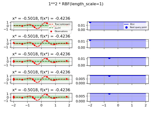
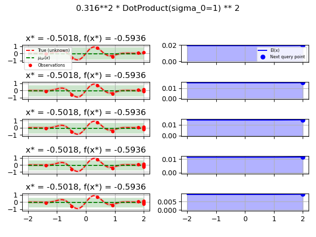
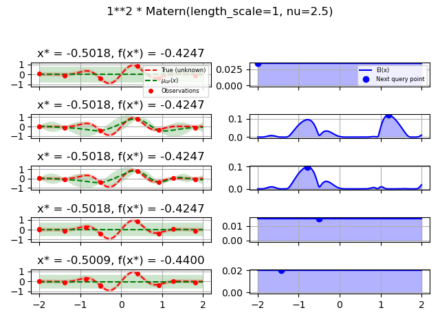
Test different kernels
from skopt.learning import GaussianProcessRegressor
from skopt.learning.gaussian_process.kernels import ConstantKernel, Matern
# Gaussian process with Matérn kernel as surrogate model
from sklearn.gaussian_process.kernels import (RBF, Matern, RationalQuadratic,
ExpSineSquared, DotProduct,
ConstantKernel)
kernels = [1.0 * RBF(length_scale=1.0, length_scale_bounds=(1e-1, 10.0)),
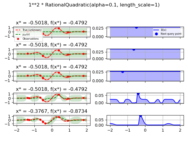
1.0 * RationalQuadratic(length_scale=1.0, alpha=0.1),
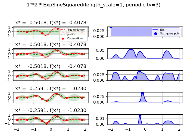
1.0 * ExpSineSquared(length_scale=1.0, periodicity=3.0,
length_scale_bounds=(0.1, 10.0),
periodicity_bounds=(1.0, 10.0)),
ConstantKernel(0.1, (0.01, 10.0))
* (DotProduct(sigma_0=1.0, sigma_0_bounds=(0.1, 10.0)) ** 2),
1.0 * Matern(length_scale=1.0, length_scale_bounds=(1e-1, 10.0),
nu=2.5)]
for kernel in kernels:
    gpr = GaussianProcessRegressor(kernel=kernel, alpha=noise_level ** 2,
                                   normalize_y=True, noise="gaussian",
                                   n_restarts_optimizer=2
                                   )
    opt = Optimizer([(-2.0, 2.0)], base_estimator=gpr, n_initial_points=5,
                    acq_optimizer="sampling", random_state=42)
    fig = plt.figure()
    fig.suptitle(repr(kernel))
    for i in range(10):
        next_x = opt.ask()
        f_val = objective(next_x)
        res = opt.tell(next_x, f_val)
        if i >= 5:
            plot_optimizer(res, n_iter=i - 5, max_iters=5)
    plt.tight_layout(rect=[0, 0.03, 1, 0.95])
    plt.show()
Total running time of the script: ( 0 minutes 8.790 seconds)
Estimated memory usage: 12 MB