Note
Click here to download the full example code or to run this example in your browser via Binder
Exploration vs exploitation
Sigurd Carlen, September 2019. Reformatted by Holger Nahrstaedt 2020
We can control how much the acqusition function favors exploration and exploitation by tweaking the two parameters kappa and xi. Higher values means more exploration and less exploitation and vice versa with low values.
kappa is only used if acq_func is set to “LCB”. xi is used when acq_func is “EI” or “PI”. By default the acqusition function is set to “gp_hedge” which chooses the best of these three. Therefore I recommend not using gp_hedge when tweaking exploration/exploitation, but instead choosing “LCB”, “EI” or “PI”.
The way to pass kappa and xi to the optimizer is to use the named argument “acq_func_kwargs”. This is a dict of extra arguments for the aqcuisition function.
If you want opt.ask() to give a new acquisition value immediately after tweaking kappa or xi call opt.update_next(). This ensures that the next value is updated with the new acquisition parameters.
This example uses plots.plot_gaussian_process which is available
since version 0.8.
print(__doc__)

import numpy as np
np.random.seed(1234)
import matplotlib.pyplot as plt
from skopt.learning import ExtraTreesRegressor
from skopt import Optimizer
from skopt.plots import plot_gaussian_process
Toy example
First we define our objective like in the ask-and-tell example notebook and define a plotting function. We do however only use on initial random point. All points after the first one is therefore chosen by the acquisition function.
noise_level = 0.1


# Our 1D toy problem, this is the function we are trying to
# minimize
def objective(x, noise_level=noise_level):
    return np.sin(5 * x[0]) * (1 - np.tanh(x[0] ** 2)) +\
           np.random.randn() * noise_level


def objective_wo_noise(x):
    return objective(x, noise_level=0)
opt = Optimizer([(-2.0, 2.0)], "GP", n_initial_points=3,
                acq_optimizer="sampling")
Plotting parameters
plot_args = {"objective": objective_wo_noise,
             "noise_level": noise_level, "show_legend": True,
             "show_title": True, "show_next_point": False,
             "show_acq_func": True}
We run a an optimization loop with standard settings
for i in range(30):
    next_x = opt.ask()
    f_val = objective(next_x)
    opt.tell(next_x, f_val)
# The same output could be created with opt.run(objective, n_iter=30)
_ = plot_gaussian_process(opt.get_result(), **plot_args)
We see that some minima is found and “exploited”
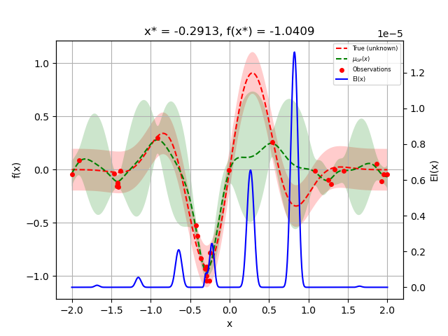
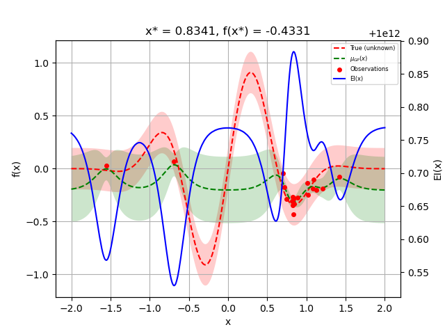
Now lets try to set kappa and xi using’to other values and pass it to the optimizer:
acq_func_kwargs = {"xi": 10000, "kappa": 10000}
opt = Optimizer([(-2.0, 2.0)], "GP", n_initial_points=3,
                acq_optimizer="sampling",
                acq_func_kwargs=acq_func_kwargs)
opt.run(objective, n_iter=20)
_ = plot_gaussian_process(opt.get_result(), **plot_args)
We see that the points are more random now.
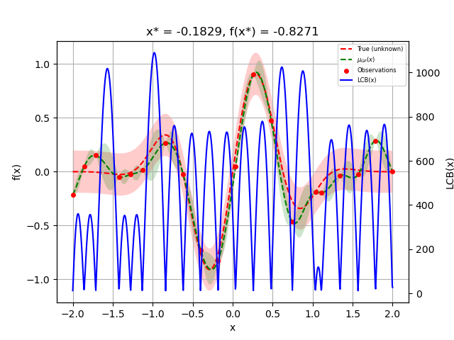
This works both for kappa when using acq_func=”LCB”:
opt = Optimizer([(-2.0, 2.0)], "GP", n_initial_points=3,
                acq_func="LCB", acq_optimizer="sampling",
                acq_func_kwargs=acq_func_kwargs)
opt.run(objective, n_iter=20)
_ = plot_gaussian_process(opt.get_result(), **plot_args)
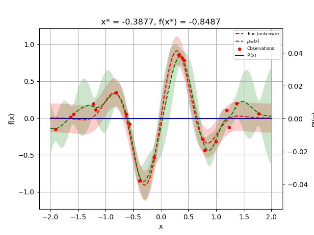
And for xi when using acq_func=”EI”: or acq_func=”PI”:
opt = Optimizer([(-2.0, 2.0)], "GP", n_initial_points=3,
                acq_func="PI", acq_optimizer="sampling",
                acq_func_kwargs=acq_func_kwargs)
opt.run(objective, n_iter=20)
_ = plot_gaussian_process(opt.get_result(), **plot_args)
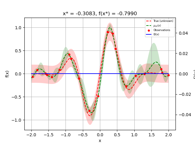
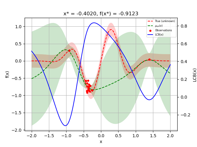
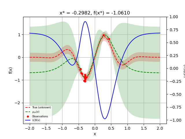
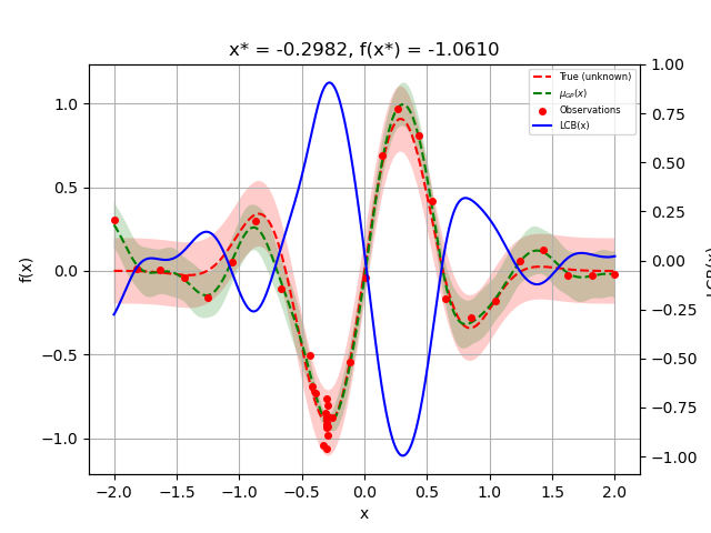
We can also favor exploitaton:
acq_func_kwargs = {"xi": 0.000001, "kappa": 0.001}
opt = Optimizer([(-2.0, 2.0)], "GP", n_initial_points=3,
                acq_func="LCB", acq_optimizer="sampling",
                acq_func_kwargs=acq_func_kwargs)
opt.run(objective, n_iter=20)
_ = plot_gaussian_process(opt.get_result(), **plot_args)
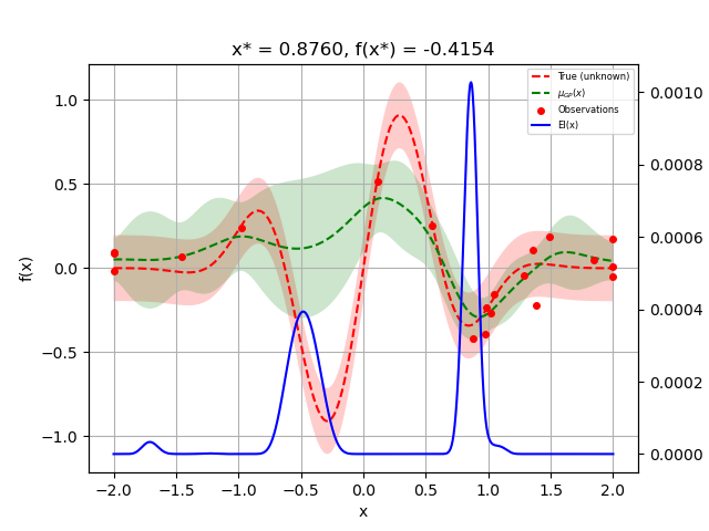
opt = Optimizer([(-2.0, 2.0)], "GP", n_initial_points=3,
                acq_func="EI", acq_optimizer="sampling",
                acq_func_kwargs=acq_func_kwargs)
opt.run(objective, n_iter=20)
_ = plot_gaussian_process(opt.get_result(), **plot_args)
opt = Optimizer([(-2.0, 2.0)], "GP", n_initial_points=3,
                acq_func="PI", acq_optimizer="sampling",
                acq_func_kwargs=acq_func_kwargs)
opt.run(objective, n_iter=20)
_ = plot_gaussian_process(opt.get_result(), **plot_args)
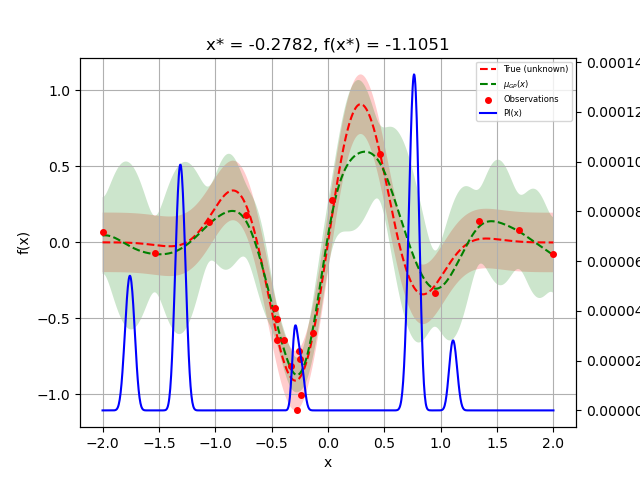
Note that negative values does not work with the “PI”-acquisition function but works with “EI”:
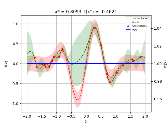
acq_func_kwargs = {"xi": -1000000000000}
opt = Optimizer([(-2.0, 2.0)], "GP", n_initial_points=3,
                acq_func="PI", acq_optimizer="sampling",
                acq_func_kwargs=acq_func_kwargs)
opt.run(objective, n_iter=20)
_ = plot_gaussian_process(opt.get_result(), **plot_args)
opt = Optimizer([(-2.0, 2.0)], "GP", n_initial_points=3,
                acq_func="EI", acq_optimizer="sampling",
                acq_func_kwargs=acq_func_kwargs)
opt.run(objective, n_iter=20)
_ = plot_gaussian_process(opt.get_result(), **plot_args)
Changing kappa and xi on the go
If we want to change kappa or ki at any point during our optimization
process we just replace opt.acq_func_kwargs. Remember to call
opt.update_next() after the change, in order for next point to be
recalculated.
acq_func_kwargs = {"kappa": 0}
opt = Optimizer([(-2.0, 2.0)], "GP", n_initial_points=3,
                acq_func="LCB", acq_optimizer="sampling",
                acq_func_kwargs=acq_func_kwargs)
opt.acq_func_kwargs
Out:
{'kappa': 0}
opt.run(objective, n_iter=20)
_ = plot_gaussian_process(opt.get_result(), **plot_args)
acq_func_kwargs = {"kappa": 100000}
opt.acq_func_kwargs = acq_func_kwargs
opt.update_next()
opt.run(objective, n_iter=20)
_ = plot_gaussian_process(opt.get_result(), **plot_args)
Total running time of the script: ( 0 minutes 29.821 seconds)
Estimated memory usage: 8 MB