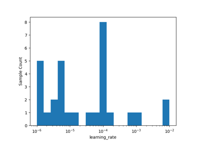
skopt.plots.plot_objective_2D
-
skopt.plots.plot_objective_2D(result, dimension_identifier1, dimension_identifier2, n_points=40, n_samples=250, levels=10, zscale='linear', sample_source='random', minimum='result', n_minimum_search=None, ax=None)[source][source]¶ Create and return a Matplotlib figure and axes with a landscape contour-plot of the last fitted model of the search-space, overlaid with all the samples from the optimization results, for the two given dimensions of the search-space.
This is similar to
plot_objective()but only for 2 dimensions whose doc-string also has a more extensive explanation.- Parameters
- result
OptimizeResult The optimization results e.g. from calling
gp_minimize().- dimension_identifier1str or int
Name or index of a dimension in the search-space.
- dimension_identifier2str or int
Name or index of a dimension in the search-space.
- n_samplesint, default=250
Number of random samples used for estimating the contour-plot of the objective function.
- n_pointsint, default=40
Number of points along each dimension where the partial dependence is evaluated when generating the contour-plots.
- levelsint, default=10
Number of levels to draw on the contour plot.
- zscalestr, default=’linear’
Scale to use for the z axis of the contour plots. Either ‘log’ or linear for all other choices.
- ax
Matplotlib.Axes, default: None When set, everything is plotted inside this axis.
- result
- Returns
- ax
Matplotlib.Axes The Matplotlib Figure-object. For example, you can save the plot by calling
fig.savefig('file.png')
- ax

