Note
Click here to download the full example code or to run this example in your browser via Binder
Comparing surrogate models
Tim Head, July 2016. Reformatted by Holger Nahrstaedt 2020
Bayesian optimization or sequential model-based optimization uses a surrogate
model to model the expensive to evaluate function func. There are several
choices for what kind of surrogate model to use. This notebook compares the
performance of:
gaussian processes,
extra trees, and
random forests
as surrogate models. A purely random optimization strategy is also used as a baseline.
print(__doc__)
import numpy as np
np.random.seed(123)
import matplotlib.pyplot as plt
Toy model
We will use the benchmarks.branin function as toy model for the expensive function.
In a real world application this function would be unknown and expensive
to evaluate.
from matplotlib.colors import LogNorm


def plot_branin():
    fig, ax = plt.subplots()

    x1_values = np.linspace(-5, 10, 100)
    x2_values = np.linspace(0, 15, 100)
    x_ax, y_ax = np.meshgrid(x1_values, x2_values)
    vals = np.c_[x_ax.ravel(), y_ax.ravel()]
    fx = np.reshape([branin(val) for val in vals], (100, 100))

    cm = ax.pcolormesh(x_ax, y_ax, fx,
                       norm=LogNorm(vmin=fx.min(),
                                    vmax=fx.max()))

    minima = np.array([[-np.pi, 12.275], [+np.pi, 2.275], [9.42478, 2.475]])
    ax.plot(minima[:, 0], minima[:, 1], "r.", markersize=14,
            lw=0, label="Minima")

    cb = fig.colorbar(cm)
    cb.set_label("f(x)")

    ax.legend(loc="best", numpoints=1)

    ax.set_xlabel("X1")
    ax.set_xlim([-5, 10])
    ax.set_ylabel("X2")
    ax.set_ylim([0, 15])


plot_branin()
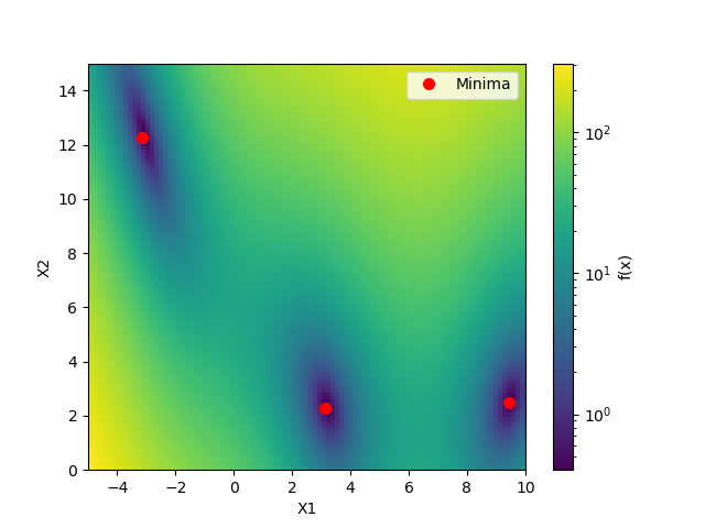
This shows the value of the two-dimensional branin function and the three minima.
Objective
The objective of this example is to find one of these minima in as
few iterations as possible. One iteration is defined as one call
to the benchmarks.branin function.
We will evaluate each model several times using a different seed for the random number generator. Then compare the average performance of these models. This makes the comparison more robust against models that get “lucky”.
from functools import partial
from skopt import gp_minimize, forest_minimize, dummy_minimize

func = partial(branin, noise_level=2.0)
bounds = [(-5.0, 10.0), (0.0, 15.0)]
n_calls = 60
def run(minimizer, n_iter=5):
    return [minimizer(func, bounds, n_calls=n_calls, random_state=n)
            for n in range(n_iter)]

# Random search
dummy_res = run(dummy_minimize)

# Gaussian processes
gp_res = run(gp_minimize)

# Random forest
rf_res = run(partial(forest_minimize, base_estimator="RF"))

# Extra trees
et_res = run(partial(forest_minimize, base_estimator="ET"))
Note that this can take a few minutes.
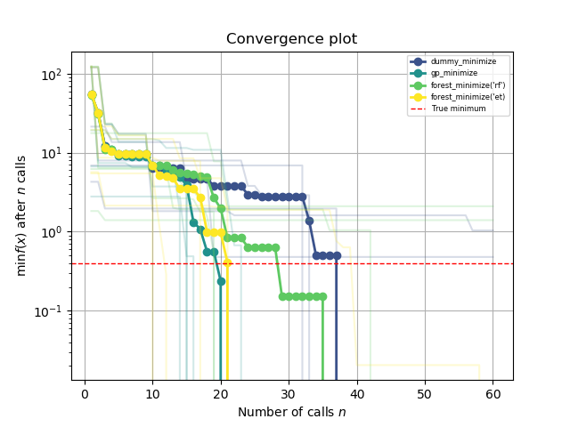
from skopt.plots import plot_convergence

plot = plot_convergence(("dummy_minimize", dummy_res),
                        ("gp_minimize", gp_res),
                        ("forest_minimize('rf')", rf_res),
                        ("forest_minimize('et)", et_res),
                        true_minimum=0.397887, yscale="log")

plot.legend(loc="best", prop={'size': 6}, numpoints=1)
Out:
<matplotlib.legend.Legend object at 0x7f8322d9f2e0>
This plot shows the value of the minimum found (y axis) as a function
of the number of iterations performed so far (x axis). The dashed red line
indicates the true value of the minimum of the benchmarks.branin function.
For the first ten iterations all methods perform equally well as they all
start by creating ten random samples before fitting their respective model
for the first time. After iteration ten the next point at which
to evaluate benchmarks.branin is guided by the model, which is where differences
start to appear.
Each minimizer only has access to noisy observations of the objective function, so as time passes (more iterations) it will start observing values that are below the true value simply because they are fluctuations.
Total running time of the script: ( 3 minutes 22.036 seconds)
Estimated memory usage: 65 MB