Note
Click here to download the full example code or to run this example in your browser via Binder
Use different base estimators for optimization
Sigurd Carlen, September 2019. Reformatted by Holger Nahrstaedt 2020
To use different base_estimator or create a regressor with different parameters, we can create a regressor object and set it as kernel.
print(__doc__)

import numpy as np
np.random.seed(1234)
import matplotlib.pyplot as plt
Toy example
Let assume the following noisy function \(f\):
x = np.linspace(-2, 2, 400).reshape(-1, 1)
fx = np.array([objective(x_i, noise_level=0.0) for x_i in x])
from skopt.acquisition import gaussian_ei

def plot_optimizer(res, next_x, x, fx, n_iter, max_iters=5):
    x_gp = res.space.transform(x.tolist())
    gp = res.models[-1]
    curr_x_iters = res.x_iters
    curr_func_vals = res.func_vals

    # Plot true function.
    ax = plt.subplot(max_iters, 2, 2 * n_iter + 1)
    plt.plot(x, fx, "r--", label="True (unknown)")
    plt.fill(np.concatenate([x, x[::-1]]),
             np.concatenate([fx - 1.9600 * noise_level,
                             fx[::-1] + 1.9600 * noise_level]),
             alpha=.2, fc="r", ec="None")
    if n_iter < max_iters - 1:
        ax.get_xaxis().set_ticklabels([])
    # Plot GP(x) + contours
    y_pred, sigma = gp.predict(x_gp, return_std=True)
    plt.plot(x, y_pred, "g--", label=r"$\mu_{GP}(x)$")
    plt.fill(np.concatenate([x, x[::-1]]),
             np.concatenate([y_pred - 1.9600 * sigma,
                             (y_pred + 1.9600 * sigma)[::-1]]),
             alpha=.2, fc="g", ec="None")

    # Plot sampled points
    plt.plot(curr_x_iters, curr_func_vals,
             "r.", markersize=8, label="Observations")
    plt.title(r"x* = %.4f, f(x*) = %.4f" % (res.x[0], res.fun))
    # Adjust plot layout
    plt.grid()

    if n_iter == 0:
        plt.legend(loc="best", prop={'size': 6}, numpoints=1)

    if n_iter != 4:
        plt.tick_params(axis='x', which='both', bottom='off',
                        top='off', labelbottom='off')

    # Plot EI(x)
    ax = plt.subplot(max_iters, 2, 2 * n_iter + 2)
    acq = gaussian_ei(x_gp, gp, y_opt=np.min(curr_func_vals))
    plt.plot(x, acq, "b", label="EI(x)")
    plt.fill_between(x.ravel(), -2.0, acq.ravel(), alpha=0.3, color='blue')

    if n_iter < max_iters - 1:
        ax.get_xaxis().set_ticklabels([])

    next_acq = gaussian_ei(res.space.transform([next_x]), gp,
                           y_opt=np.min(curr_func_vals))
    plt.plot(next_x, next_acq, "bo", markersize=6, label="Next query point")

    # Adjust plot layout
    plt.ylim(0, 0.07)
    plt.grid()
    if n_iter == 0:
        plt.legend(loc="best", prop={'size': 6}, numpoints=1)

    if n_iter != 4:
        plt.tick_params(axis='x', which='both', bottom='off',
                        top='off', labelbottom='off')
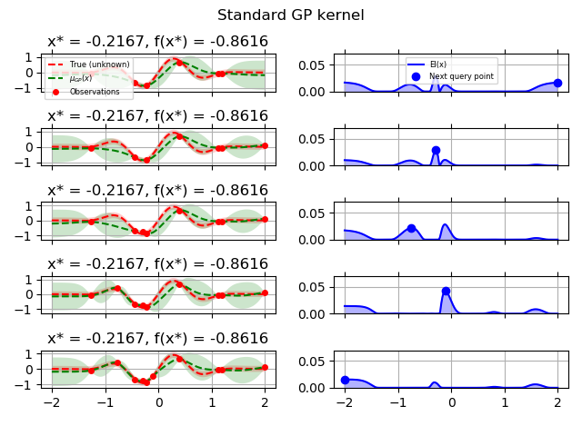
GP kernel
fig = plt.figure()
fig.suptitle("Standard GP kernel")
for i in range(10):
    next_x = opt_gp.ask()
    f_val = objective(next_x)
    res = opt_gp.tell(next_x, f_val)
    if i >= 5:
        plot_optimizer(res, opt_gp._next_x, x, fx, n_iter=i-5, max_iters=5)
plt.tight_layout(rect=[0, 0.03, 1, 0.95])
plt.plot()
Out:
[]
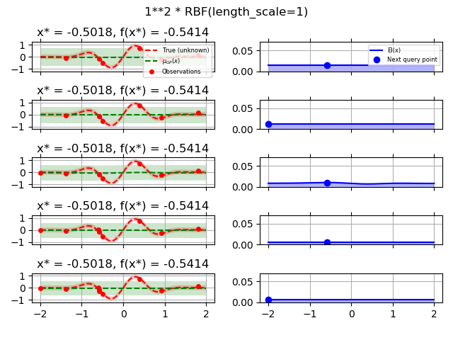
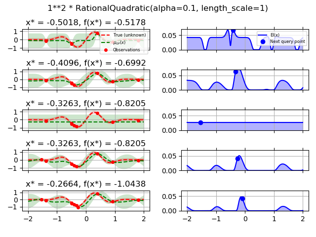
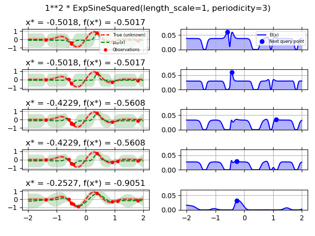
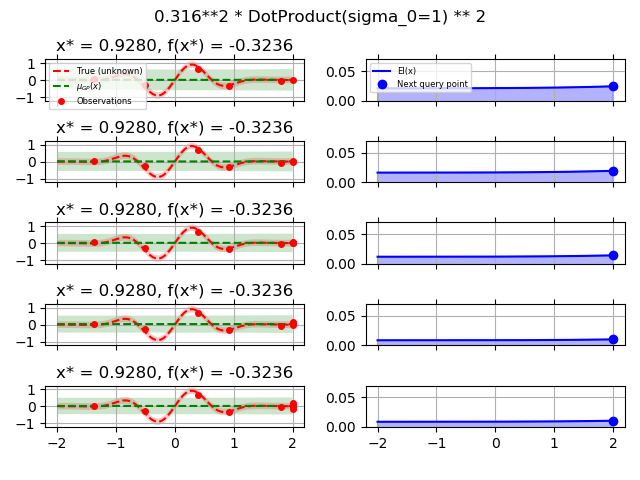
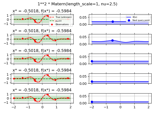
Test different kernels
from skopt.learning import GaussianProcessRegressor
from skopt.learning.gaussian_process.kernels import ConstantKernel, Matern
# Gaussian process with Matérn kernel as surrogate model

from sklearn.gaussian_process.kernels import (RBF, Matern, RationalQuadratic,
                                              ExpSineSquared, DotProduct,
                                              ConstantKernel)


kernels = [1.0 * RBF(length_scale=1.0, length_scale_bounds=(1e-1, 10.0)),
           1.0 * RationalQuadratic(length_scale=1.0, alpha=0.1),
           1.0 * ExpSineSquared(length_scale=1.0, periodicity=3.0,
                                length_scale_bounds=(0.1, 10.0),
                                periodicity_bounds=(1.0, 10.0)),
           ConstantKernel(0.1, (0.01, 10.0))
               * (DotProduct(sigma_0=1.0, sigma_0_bounds=(0.1, 10.0)) ** 2),
           1.0 * Matern(length_scale=1.0, length_scale_bounds=(1e-1, 10.0),
                        nu=2.5)]
for kernel in kernels:
    gpr = GaussianProcessRegressor(kernel=kernel, alpha=noise_level ** 2,
                                   normalize_y=True, noise="gaussian",
                                   n_restarts_optimizer=2
                                   )
    opt = Optimizer([(-2.0, 2.0)], base_estimator=gpr, n_initial_points=5,
                    acq_optimizer="sampling", random_state=42)
    fig = plt.figure()
    fig.suptitle(repr(kernel))
    for i in range(10):
        next_x = opt.ask()
        f_val = objective(next_x)
        res = opt.tell(next_x, f_val)
        if i >= 5:
            plot_optimizer(res, opt._next_x, x, fx, n_iter=i - 5, max_iters=5)
    plt.tight_layout(rect=[0, 0.03, 1, 0.95])
    plt.show()
Total running time of the script: ( 0 minutes 9.161 seconds)
Estimated memory usage: 13 MB