Note
Click here to download the full example code or to run this example in your browser via Binder
Async optimization Loop
Bayesian optimization is used to tune parameters for walking robots or other experiments that are not a simple (expensive) function call.
Tim Head, February 2017. Reformatted by Holger Nahrstaedt 2020
They often follow a pattern a bit like this:
ask for a new set of parameters
walk to the experiment and program in the new parameters
observe the outcome of running the experiment
walk back to your laptop and tell the optimizer about the outcome
go to step 1
A setup like this is difficult to implement with the *_minimize() function interface. This is why scikit-optimize has a ask-and-tell interface that you can use when you want to control the execution of the optimization loop.
This notebook demonstrates how to use the ask and tell interface.
print(__doc__)

import numpy as np
np.random.seed(1234)

import matplotlib.pyplot as plt
The Setup
We will use a simple 1D problem to illustrate the API. This is a little bit artificial as you normally would not use the ask-and-tell interface if you had a function you can call to evaluate the objective.
from skopt.learning import ExtraTreesRegressor
from skopt import Optimizer

noise_level = 0.1
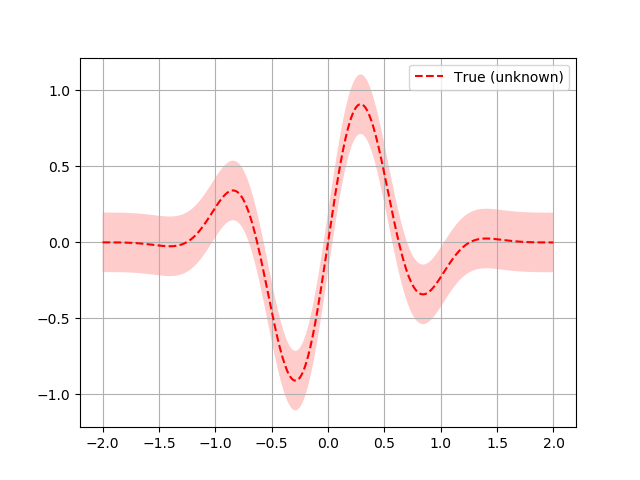
Our 1D toy problem, this is the function we are trying to minimize
Here a quick plot to visualize what the function looks like:
# Plot f(x) + contours
plt.set_cmap("viridis")
x = np.linspace(-2, 2, 400).reshape(-1, 1)
fx = np.array([objective(x_i, noise_level=0.0) for x_i in x])
plt.plot(x, fx, "r--", label="True (unknown)")
plt.fill(np.concatenate([x, x[::-1]]),
         np.concatenate(([fx_i - 1.9600 * noise_level for fx_i in fx],
                         [fx_i + 1.9600 * noise_level for fx_i in fx[::-1]])),
         alpha=.2, fc="r", ec="None")
plt.legend()
plt.grid()
plt.show()
Now we setup the Optimizer class. The arguments follow the meaning and
naming of the *_minimize() functions. An important difference is that
you do not pass the objective function to the optimizer.
opt = Optimizer([(-2.0, 2.0)], "ET", acq_optimizer="sampling")

# To obtain a suggestion for the point at which to evaluate the objective
# you call the ask() method of opt:

next_x = opt.ask()
print(next_x)
Out:
[-1.7121321838148869]
In a real world use case you would probably go away and use this parameter in your experiment and come back a while later with the result. In this example we can simply evaluate the objective function and report the value back to the optimizer:
f_val = objective(next_x)
opt.tell(next_x, f_val)
Out:
         fun: -0.032758350111535384
   func_vals: array([-0.03275835])
      models: []
random_state: RandomState(MT19937) at 0x7F833EAFAD40
       space: Space([Real(low=-2.0, high=2.0, prior='uniform', transform='identity')])
       specs: None
           x: [-1.7121321838148869]
     x_iters: [[-1.7121321838148869]]
Like *_minimize() the first few points are random suggestions as there is no data yet with which to fit a surrogate model.
for i in range(9):
    next_x = opt.ask()
    f_val = objective(next_x)
    opt.tell(next_x, f_val)
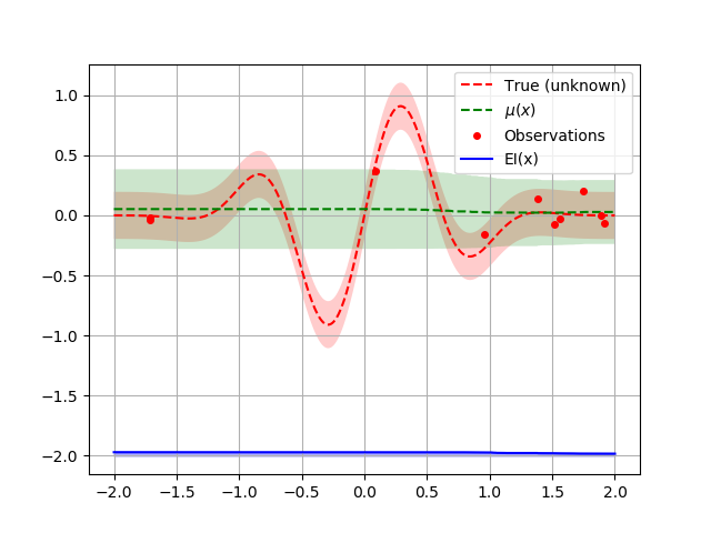
We can now plot the random suggestions and the first model that has been fit:
from skopt.acquisition import gaussian_ei


def plot_optimizer(opt, x, fx):
    model = opt.models[-1]
    x_model = opt.space.transform(x.tolist())

    # Plot true function.
    plt.plot(x, fx, "r--", label="True (unknown)")
    plt.fill(np.concatenate([x, x[::-1]]),
             np.concatenate([fx - 1.9600 * noise_level,
                             fx[::-1] + 1.9600 * noise_level]),
             alpha=.2, fc="r", ec="None")

    # Plot Model(x) + contours
    y_pred, sigma = model.predict(x_model, return_std=True)
    plt.plot(x, y_pred, "g--", label=r"$\mu(x)$")
    plt.fill(np.concatenate([x, x[::-1]]),
             np.concatenate([y_pred - 1.9600 * sigma,
                             (y_pred + 1.9600 * sigma)[::-1]]),
             alpha=.2, fc="g", ec="None")

    # Plot sampled points
    plt.plot(opt.Xi, opt.yi,
             "r.", markersize=8, label="Observations")

    acq = gaussian_ei(x_model, model, y_opt=np.min(opt.yi))
    # shift down to make a better plot
    acq = 4 * acq - 2
    plt.plot(x, acq, "b", label="EI(x)")
    plt.fill_between(x.ravel(), -2.0, acq.ravel(), alpha=0.3, color='blue')

    # Adjust plot layout
    plt.grid()
    plt.legend(loc='best')


plot_optimizer(opt, x, fx)
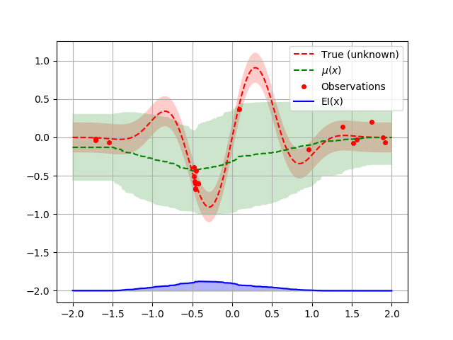
Let us sample a few more points and plot the optimizer again:
for i in range(10):
    next_x = opt.ask()
    f_val = objective(next_x)
    opt.tell(next_x, f_val)

plot_optimizer(opt, x, fx)
By using the Optimizer class directly you get control over the
optimization loop.
You can also pickle your Optimizer instance if you want to end the
process running it and resume it later. This is handy if your experiment
takes a very long time and you want to shutdown your computer in the
meantime:
import pickle

with open('my-optimizer.pkl', 'wb') as f:
    pickle.dump(opt, f)

with open('my-optimizer.pkl', 'rb') as f:
    opt_restored = pickle.load(f)
Total running time of the script: ( 0 minutes 5.175 seconds)
Estimated memory usage: 8 MB